Getting started with CAMS • interactmeta

This vignette is the short path to cams(): estimands, assumptions, Bayesian and REML inference on the same model, and the main summaries. Contribution-adjusted meta-analysis (CAMS) is the treatment-by-subgroup interaction model developed in Panaro et al. (2025). For additional shipped datasets (age, edss, il6, RESPIRE), see vignette("worked-examples"). For tables you can QC or hand to reporting, see vignette("export-and-qc").

Estimands (what CAMS reports)

Estimand	Function	Depends on reporting IF?
Treatment-by-subgroup interaction $\gamma$	`interactions()`	No
Modifier-level mean effects $\mu_A(\pi)$ , $\mu_B(\pi)$	`modifiers()`	Yes (default pooled $\widetilde{\pi}$ )
Combined-population mean $M(\pi)$	`combined()`	Yes
Trial information fractions $\pi_j$	`ifrac()` (optional before fit)	Built inside `cams()` by default

The reference modifier (e.g. NIV vs IV) sets the direction of $\gamma$ . All fits are on the escalc scale (yi, vi); use exponentiate = TRUE for odds ratios, hazard ratios, or other ratio measures.

Scope and key assumptions

Intended use. CAMS synthesises aggregate subgroup effects across trials (published tables, systematic reviews, HTA-style evidence pools). It is not a substitute for a pre-specified subgroup analysis in a single randomised trial SAP.

Data. Long format: one row per trial × modifier with yi and vi. Use escalc() (re-exported from metafor (Viechtbauer 2010)) when starting from event counts.

Within-trial sampling. The implementation treats the two modifier estimates in a trial as conditionally independent with variances vi, and uses precision-based information fractions $\pi_j$ . Shared control arms, nested subgroups, or other within-trial dependence are not modelled yet (see ?cams, section on sampling assumption).

Between-trial heterogeneity. Separate random-effects components for the interaction contrasts and the combined-effect meta-regression (Panaro et al. 2025); see heterogeneity() after fit.

Example: COVID steroids (IV / NIV)

The steroids data are mortality odds ratios by ventilation subgroup (IV vs NIV) from the REACT meta-analysis (WHO Rapid Evidence Appraisal for COVID-19 Therapies (REACT) Working Group et al. 2020). Rows with n = 0 mark unreported subgroups; ifrac() completes the table for CAMS (see vignette("worked-examples"), il6 section).

library(interactmeta)
library(dplyr)

steroids_obs <- steroids |> filter(n > 0)
steroids_es <- escalc(
  measure = "OR",
  ai = treat.events,
  bi = treat.total - treat.events,
  ci = cont.events,
  di = cont.total - cont.events,
  data = steroids_obs
)
des <- ifrac(steroids_es, reference = "NIV")

One model, two inference backends

cams() specifies the same CAMS likelihood; choose Bayesian (default, bayesmeta (Röver 2020)) or frequentist (method = "REML", metafor (Viechtbauer 2010)). Below we fit both on des with reference = "NIV". The half-normal scales on $\tau_m$ and $\tau_g$ follow Panaro et al. (2026a) (not the package defaults, which are improper uniform priors on heterogeneity).

fit_bayes <- cams(
  des,
  reference = "NIV",
  tau.prior = function(tau) bayesmeta::dhalfnormal(tau, scale = 0.5),
  tau.interaction.prior = function(tau) bayesmeta::dhalfnormal(tau, scale = 0.1)
)
fit_reml <- cams(des, reference = "NIV", method = "REML")

The interaction does not depend on the reporting information fraction. Modifier and combined summaries do; they use the pooled reporting $\widetilde{\pi}$ from ifrac(fit) by default.

ix_b <- tidy(interactions(fit_bayes, type = "Overall", exponentiate = TRUE))
ix_r <- tidy(interactions(fit_reml, type = "Overall", exponentiate = TRUE))
knitr::kable(
  bind_rows(Bayesian = ix_b, REML = ix_r, .id = "inference") |>
    select(inference, type, estimate, conf.low, conf.high),
  digits = 2,
  caption = "Interaction (OR scale): Bayesian credible vs REML confidence intervals"
)

Interaction (OR scale): Bayesian credible vs REML confidence intervals
inference	type	estimate	conf.low	conf.high
Bayesian	Overall	1.35	0.32	2.38
REML	Overall	1.35	0.32	2.38

Bayesian and REML CAMS intervals are comparable. Bayesian credible intervals use the DIRECT quadrature mixture (Röver and Friede 2017); they reflect heterogeneity uncertainty and the priors above. REML intervals are Wald confidence intervals from the stored metafor fit (Viechtbauer 2010).

interactions(fit_reml, type = "Overall", exponentiate = TRUE)
#> interaction  type     estimate    se  Overall 95% CI
#> IV-NIV       Overall      1.35  0.52    (0.32, 2.38)
modifiers(fit_reml, type = "Overall", exponentiate = TRUE)
#> level  type     estimate    se  Overall 95% CI
#>    IV  Overall      1.47  0.47    (0.78, 2.77)
#>   NIV  Overall      0.38  0.15    (0.18, 0.82)
combined(fit_reml, type = "Overall", exponentiate = TRUE)
#> combined  estimate    se  Overall 95% CI
#>      All     -0.16  0.79   (-1.72, 1.39)
ifrac(fit_reml, ifrac = "interaction")
#>                   IF  estimate
#> interaction-weighted      0.59
#> (at fitted interaction heterogeneity τ_γ)

Forest plot (reporting checklist)

forestplot() draws observed modifier estimates, optional shrinkage, and Overall / Prediction summaries at $\widetilde{\pi}$ . For publication-style figures, set exponentiate = TRUE, favours text, and keep table numbers from tidy(modifiers(...)) aligned with the pooled diamonds.

forestplot(
  fit_reml,
  exponentiate = TRUE,
  favours = c("Lower mortality", "Higher mortality")
)

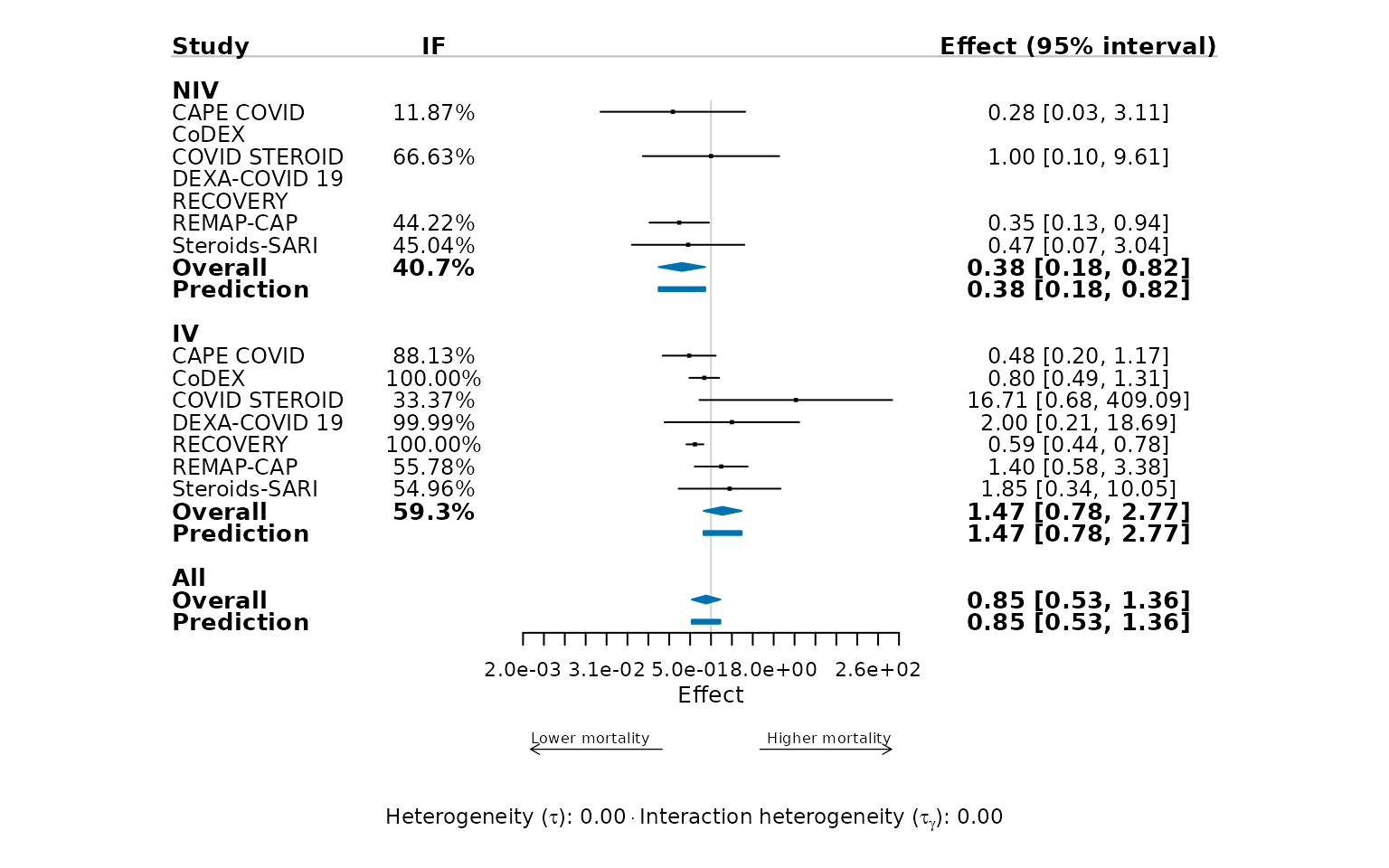
Caption ingredients: population (critically ill COVID-19), estimand (OR for mortality by ventilation subgroup), CAMS with method = "REML", reference NIV, reporting IF from ifrac(fit_reml), interval type (Wald CI for REML).

Next steps

Sensitivity to other constructions: da(), ad(), and swada() (DA and AD are distinct estimators (Panaro et al. 2026b); see also Fisher et al. (2017)), plus compare() on sensitivity() output — worked in vignette("export-and-qc").
Other datasets: vignette("worked-examples").

References

Fisher, David J., James R. Carpenter, Tim P. Morris, Suzanne C. Freeman, and Jayne F. Tierney. 2017. “Meta-Analytical Methods to Identify Who Benefits Most from Treatments: Daft, Deluded, or Deft Approach?” BMJ 356: j573.

Panaro, Renato Valladares, Christian Röver, and Tim Friede. 2025. “Consistent Bayesian Meta-Analysis on Subgroup Specific Effects and Interactions.” arXiv Preprint arXiv:2512.18785. https://arxiv.org/abs/2512.18785.

Panaro, Renato Valladares, Christian Röver, and Tim Friede. 2026a. “Empirical Prior Distributions for Treatment-by-Subgroup Interaction Heterogeneity in Random-Effects Meta-Analysis.” arXiv Preprint arXiv:2606.23968. https://arxiv.org/abs/2606.23968.

Panaro, Renato Valladares, Christian Röver, and Tim Friede. 2026b. “Subgroup Comparisons Within and Across Studies in Meta-Analysis.” Research Synthesis Methods. https://arxiv.org/abs/2508.15531.

Röver, Christian. 2020. “Bayesian Random-Effects Meta-Analysis Using the Bayesmeta R Package.” Journal of Statistical Software 93 (6): 1–51. https://doi.org/10.18637/jss.v093.i06.

Röver, Christian, and Tim Friede. 2017. “Discrete Approximation of a Mixture Distribution via Restricted Divergence.” Journal of Computational and Graphical Statistics 26 (1): 217–22.

Viechtbauer, Wolfgang. 2010. “Conducting Meta-Analyses in R with the Metafor Package.” Journal of Statistical Software 36 (3): 1–48. https://doi.org/10.18637/jss.v036.i03.

WHO Rapid Evidence Appraisal for COVID-19 Therapies (REACT) Working Group, Jonathan A. C. Sterne, Srinivas Murthy, et al. 2020. “Association Between Administration of Systemic Corticosteroids and Mortality Among Critically Ill Patients with COVID-19: A Meta-Analysis.” JAMA 324 (13): 1330–41.