Bayesian fits use the same Stan likelihood as MLE
but sample from the posterior with rstan::sampling.
Before you model
Brief exploratory context for the larynx data (see Getting started for full EDA):
library(spsurv)
library(generics)
library(KMsurv)
library(survival)
library(ggplot2)
data(larynx)
larynx$stage <- factor(larynx$stage)
km_stage <- survfit(Surv(time, delta) ~ stage, data = larynx)
km_long <- data.frame(
  time = km_stage$time,
  surv = km_stage$surv,
  stage = rep(levels(larynx$stage), km_stage$strata)
)
ggplot(km_long, aes(x = time, y = surv, color = stage)) +
  geom_step(linewidth = 0.6) +
  labs(x = "Time (years)", y = "Survival probability", color = "Stage") +
  theme_bw() +
  theme(legend.position = "bottom")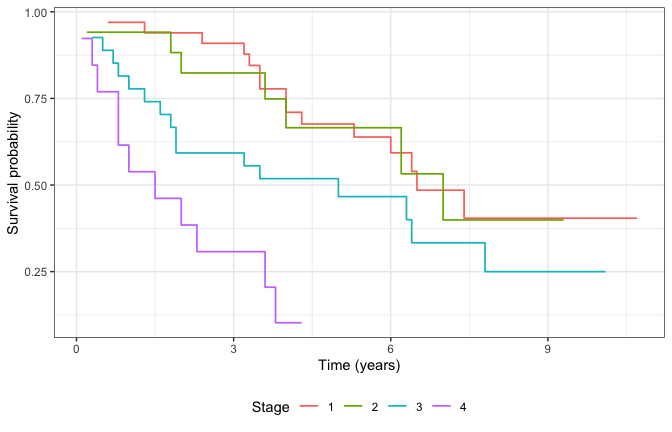
Kaplan-Meier by stage (unadjusted).
Fit and summarize
fit <- bpph(
  Surv(time, delta) ~ age + stage,
  degree = 5,
  data = larynx,
  approach = "bayes",
  iter = 400,
  warmup = 200,
  chains = 1,
  cores = 1,
  init = 0,
  priors = list(
    beta = c("normal(0,4)"),
    gamma = c("lognormal(0,4)")
  )
)
#>
#> SAMPLING FOR MODEL 'spbp' NOW (CHAIN 1).
#> Chain 1:
#> Chain 1: Gradient evaluation took 7e-05 seconds
#> Chain 1: 1000 transitions using 10 leapfrog steps per transition would take 0.7 seconds.
#> Chain 1: Adjust your expectations accordingly!
#> Chain 1:
#> Chain 1:
#> Chain 1: Iteration:   1 / 400 [  0%]  (Warmup)
#> Chain 1: Iteration:  40 / 400 [ 10%]  (Warmup)
#> Chain 1: Iteration:  80 / 400 [ 20%]  (Warmup)
#> Chain 1: Iteration: 120 / 400 [ 30%]  (Warmup)
#> Chain 1: Iteration: 160 / 400 [ 40%]  (Warmup)
#> Chain 1: Iteration: 200 / 400 [ 50%]  (Warmup)
#> Chain 1: Iteration: 201 / 400 [ 50%]  (Sampling)
#> Chain 1: Iteration: 240 / 400 [ 60%]  (Sampling)
#> Chain 1: Iteration: 280 / 400 [ 70%]  (Sampling)
#> Chain 1: Iteration: 320 / 400 [ 80%]  (Sampling)
#> Chain 1: Iteration: 360 / 400 [ 90%]  (Sampling)
#> Chain 1: Iteration: 400 / 400 [100%]  (Sampling)
#> Chain 1:
#> Chain 1:  Elapsed Time: 0.166 seconds (Warm-up)
#> Chain 1:                0.186 seconds (Sampling)
#> Chain 1:                0.352 seconds (Total)
#> Chain 1:
summary(fit)
#> Call:
#> bpph(formula = Surv(time, delta) ~ age + stage, degree = 5, data = larynx,
#>     approach = "bayes", iter = 400, warmup = 200, chains = 1,
#>     cores = 1, init = 0, priors = list(beta = c("normal(0,4)"),
#>         gamma = c("lognormal(0,4)")), model = "ph")
#>
#> Bayesian Bernstein PH model:
#> Regression coefficients:
#>        Estimate    2.5%   97.5% Std. Error
#> age      0.0233 -0.0087  0.0480        0.0
#> stage2   0.1219 -0.7143  0.9710        0.5
#> stage3   0.6059 -0.3214  1.2143        0.4
#> stage4   1.6720  0.7426  2.5565        0.4
#>
#> Exponentiated coefficients:
#>        Estimate 2.5% 97.5%
#> age        1.02 0.99   1.0
#> stage2     1.25 0.40   2.3
#> stage3     1.97 0.73   3.4
#> stage4     5.87 1.52  11.2
#>
#> ---
#> DIC = 296 WAIC = -149Visual check — posterior forest plot
td_b <- tidy(fit, conf.int = TRUE, exponentiate = TRUE)
hpd <- credint(fit, prob = 0.95, type = "HPD")
td_b$hpd.low <- exp(hpd[, 1])
td_b$hpd.high <- exp(hpd[, 2])
td_b$term <- factor(td_b$term, levels = rev(td_b$term))

ggplot(td_b, aes(x = estimate, y = term)) +
  geom_vline(xintercept = 1, linetype = "dashed", color = "grey50") +
  geom_pointrange(aes(xmin = hpd.low, xmax = hpd.high), linewidth = 0.4, color = "steelblue") +
  labs(x = "Hazard ratio (posterior median)", y = NULL, title = "95% HPD intervals") +
  theme_bw()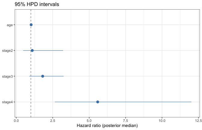
Posterior medians with 95% HPD intervals (exponentiated).
Visual check — MLE vs Bayes
td_m <- tidy(fit_mle, conf.int = TRUE, exponentiate = TRUE)
cmp <- merge(
  td_m[, c("term", "estimate", "conf.low", "conf.high")],
  td_b[, c("term", "estimate", "hpd.low", "hpd.high")],
  by = "term",
  suffixes = c("_mle", "_bayes")
)
cmp_long <- rbind(
  data.frame(term = cmp$term, method = "MLE", low = cmp$conf.low, high = cmp$conf.high,
             est = cmp$estimate_mle),
  data.frame(term = cmp$term, method = "Bayes", low = cmp$hpd.low, high = cmp$hpd.high,
             est = cmp$estimate_bayes)
)
cmp_long$term <- factor(cmp_long$term, levels = rev(unique(cmp$term)))

ggplot(cmp_long, aes(x = est, y = term, color = method)) +
  geom_vline(xintercept = 1, linetype = "dashed", color = "grey50") +
  geom_pointrange(aes(xmin = low, xmax = high), position = position_dodge(width = 0.5), linewidth = 0.4) +
  labs(x = "Hazard ratio", y = NULL, color = NULL) +
  theme_bw()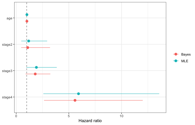
MLE 95% CI vs Bayesian 95% HPD (exponentiated).
Credible intervals and criteria
credint(fit, prob = 0.95, type = "HPD")
#>               lower      upper
#> age    -0.008682201 0.04795021
#> stage2 -0.714296360 0.97097272
#> stage3 -0.321423136 1.21432591
#> stage4  0.742574440 2.55648825
#> attr(,"Probability")
#> [1] 0.95Convergence (optional deep dive)
Install bayesplot for trace and pairs plots:
Always inspect divergences, split R-hat, and ESS before interpreting results.
tidybayes posterior draws
Install posterior and tidybayes for
long-format draws and interval plots. After
library(spsurv), spread_draws() and
tidy_draws() dispatch on Bayes fits when
tidybayes is loaded.
library(tidybayes)
dr <- as_draws_df.spbp(fit)
spread_draws(fit, `beta[age]`)
#> # A tibble: 200 × 4
#>    .chain .iteration .draw `beta[age]`
#>     <int>      <int> <int>       <dbl>
#>  1      1          1     1    0.0536
#>  2      1          2     2    0.00867
#>  3      1          3     3   -0.00540
#>  4      1          4     4    0.0235
#>  5      1          5     5   -0.000776
#>  6      1          6     6    0.0117
#>  7      1          7     7    0.0568
#>  8      1          8     8    0.0333
#>  9      1          9     9    0.00501
#> 10      1         10    10    0.0436
#> # ℹ 190 more rows
Draw-level survival curves:
head(spread_surv_draws.spbp(fit, times = c(1, 2, 3), newdata = larynx[1, ]))
#>     stage time age diagyr delta .chain .iteration .draw time      surv id
#> 1       1  0.6  77     76     1      1          1     1    1 0.9280900  1
#> 1.1     1  0.6  77     76     1      1          1     1    2 0.8339741  1
#> 1.2     1  0.6  77     76     1      1          1     1    3 0.7102063  1
#> 1.3     1  0.6  77     76     1      1          2     2    1 0.9349245  1
#> 1.4     1  0.6  77     76     1      1          2     2    2 0.8823173  1
#> 1.5     1  0.6  77     76     1      1          2     2    3 0.8301550  1
See vignette("tidymodels", package = "spsurv") for
workflows and parsnip engines.
Survival prediction
Posterior mean survival is a Bernstein polynomial in time, so the
curve is smooth (geom_line). Kaplan–Meier
in the EDA plot above remains a step function.
pr <- predict(fit, times = seq(0, max(larynx$time), length.out = 121))
head(pr)
#>   id       time      surv     lower     upper     cumhaz     std.err
#> 1  1 0.00000000 1.0000000 1.0000000 1.0000000 0.00000000 0.000000000
#> 2  1 0.08916667 0.9890259 0.9822037 0.9961573 0.01104205 0.003772371
#> 3  1 0.17833333 0.9783350 0.9652800 0.9923706 0.02193037 0.007230845
#> 4  1 0.26750000 0.9679095 0.9472842 0.9860674 0.03267434 0.010401111
#> 5  1 0.35666667 0.9577324 0.9309257 0.9809029 0.04328328 0.013307143
#> 6  1 0.44583333 0.9477880 0.9146768 0.9740549 0.05376647 0.015971283
ggplot(pr, aes(x = time, y = surv)) +
  geom_ribbon(aes(ymin = lower, ymax = upper), alpha = 0.2, colour = NA) +
  geom_line(linewidth = 0.6) +
  labs(x = "Time (years)", y = "Survival probability") +
  theme_bw()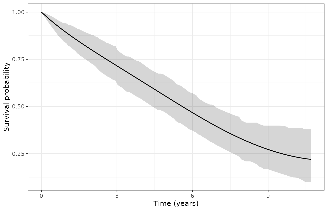
Smooth posterior survival at the mean covariate profile with 95% HPD ribbon.
See the Survival prediction and ggplot vignette for covariate-specific ribbons.