Bernstein polynomial degree and baseline plots

The unknown baseline is approximated by a Bernstein polynomial of degree m. The vector bp.param holds the m baseline coefficients (gamma).

Before you model

library(spsurv)
library(survival)
library(ggplot2)
data(veteran)

ggplot(subset(veteran, status == 1), aes(x = time)) +
  geom_histogram(bins = 25, fill = "steelblue", color = "white", alpha = 0.8) +
  labs(x = "Time (days)", y = "Count", title = "Event times only") +
  theme_bw()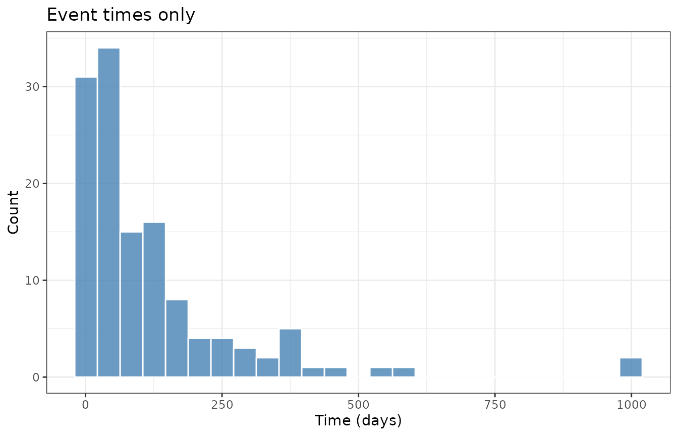

Distribution of observed event times.

The support of event times motivates the upper limit tau used in Bernstein basis evaluation (max(time) by default).

Why this is insightful

Sparse events at long follow-up times limit how wiggly a high-degree baseline can be estimated reliably.

What to decide

• Very few late events → prefer moderate degree; inspect baseline smoothness.

Fit and summarize

fit_low <- bpph(
  Surv(time, status) ~ karno,
  degree = 3,
  data = veteran,
  approach = "mle",
  init = 0
)
fit_high <- bpph(
  Surv(time, status) ~ karno,
  degree = 8,
  data = veteran,
  approach = "mle",
  init = 0
)
c(low = length(fit_low$bp.param), high = length(fit_high$bp.param))
#>  low high 
#>    3    8

AIC(fit_low, fit_high)
#>      fit model degree      aic npars
#> 1 model1    ph      3 1458.842     4
#> 2 model2    ph      8 1465.575     9

Visual check — baseline overlay

times <- seq(0, max(veteran$time), length.out = 100)
tau <- max(veteran$time)

baseline_curve <- function(fit, times, tau) {
  bb <- bp.basis(times, degree = length(fit$bp.param), tau = tau)
  data.frame(
    time = times,
    cumhaz = as.vector(bb$G %*% fit$bp.param),
    degree = paste0("m = ", length(fit$bp.param))
  )
}

bl_df <- rbind(
  baseline_curve(fit_low, times, tau),
  baseline_curve(fit_high, times, tau)
)

ggplot(bl_df, aes(x = time, y = cumhaz, color = degree)) +
  geom_line(linewidth = 0.7) +
  labs(x = "Time (days)", y = "Cumulative baseline hazard", color = NULL) +
  theme_bw()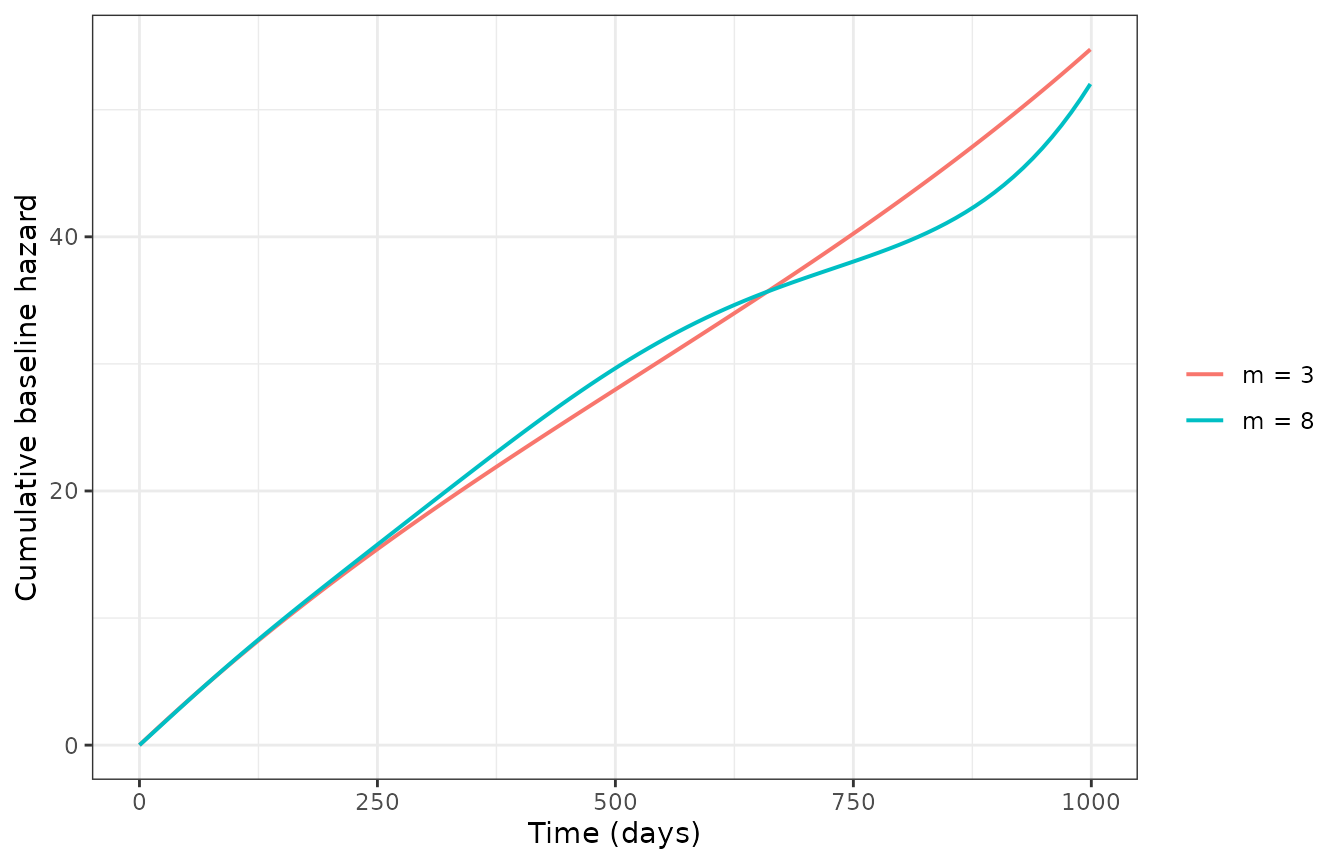

Cumulative baseline hazard: degree 3 vs degree 8.

plot(fit_high, graph = "baseline", cumulative = FALSE)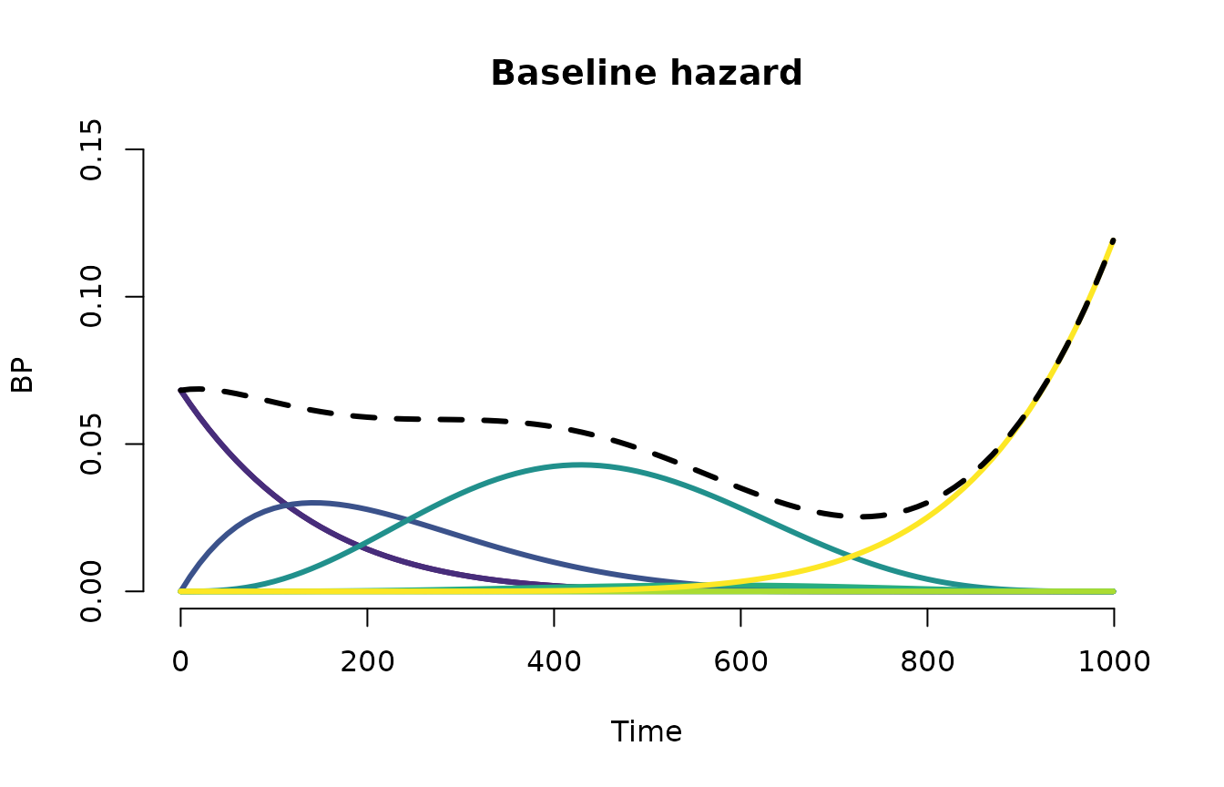

Estimated baseline hazard components (degree 8).

plot(fit_high, graph = "basis", cumulative = FALSE)

Bernstein basis functions on [0, tau].

Why this is insightful

A wiggly high-degree baseline is an overfitting signal. Flat or unstable AIC combined with high gamma condition numbers suggests reducing m.

What to decide

• Oscillating baseline hazard → lower degree.
• AIC improves but kappa explodes → prefer parsimony; bands may be unreliable.
• Stable baseline shape across nearby degrees → degree choice is robust.

Gamma information stability

kappa_tbl <- data.frame(
  degree = c(3, 8),
  gamma_information_stable = c(
    attr(vcov(fit_low, bp.param = TRUE), "gamma_information_stable"),
    attr(vcov(fit_high, bp.param = TRUE), "gamma_information_stable")
  ),
  kappa_gamma = c(
    signif(attr(vcov(fit_low, bp.param = TRUE), "gamma_information_kappa"), 4),
    signif(attr(vcov(fit_high, bp.param = TRUE), "gamma_information_kappa"), 4)
  )
)
kappa_tbl
#>   degree gamma_information_stable kappa_gamma
#> 1      3                     TRUE   1.460e+02
#> 2      8                    FALSE   8.236e+10

Basis functions

times <- seq(0, max(veteran$time), length.out = 50)
bb <- bp.basis(times, degree = 5, tau = max(veteran$time))
dim(bb$g)
#> [1] 50  5

For AFT models, the internal power-basis matrix comes from pw.basis():

pw <- pw.basis(degree = 5)
dim(pw)
#> [1] 5 5