spsurv fits semi-parametric survival regression for right-censored data using Bernstein-polynomial (BP) baselines. Three model families share one interface:
-
PH — proportional hazards (
bpph,model = "ph") -
PO — proportional odds (
bppo,model = "po") -
AFT — accelerated failure time (
bpaft,model = "aft")
Before you model
library(spsurv)
library(KMsurv)
library(survival)
library(ggplot2)
library(generics)
data(larynx)
larynx$stage <- factor(larynx$stage)
censor_tbl <- do.call(rbind, lapply(split(larynx, larynx$stage), function(d) {
  data.frame(
    stage = as.character(d$stage[1]),
    n = nrow(d),
    events = sum(d$delta),
    censored = sum(1 - d$delta),
    stringsAsFactors = FALSE
  )
}))
censor_tbl$pct_censored <- round(100 * censor_tbl$censored / censor_tbl$n, 1)
censor_tbl
#>   stage  n events censored pct_censored
#> 1     1 33     15       18         54.5
#> 2     2 17      7       10         58.8
#> 3     3 27     17       10         37.0
#> 4     4 13     11        2         15.4
km_stage <- survfit(Surv(time, delta) ~ stage, data = larynx)
km_long <- data.frame(
  time = km_stage$time,
  surv = km_stage$surv,
  stage = rep(levels(larynx$stage), km_stage$strata)
)
ggplot(km_long, aes(x = time, y = surv, color = stage)) +
  geom_step(linewidth = 0.6) +
  labs(x = "Time (years)", y = "Survival probability", color = "Stage") +
  theme_bw() +
  theme(legend.position = "bottom")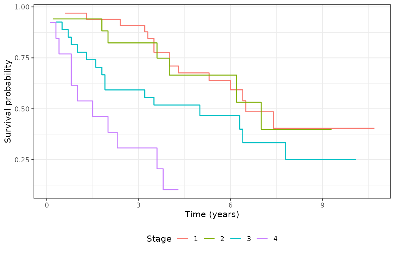
Kaplan-Meier survival by larynx cancer stage.
Fit and summarize
fit <- bpph(
  Surv(time, delta) ~ age + stage,
  degree = 5,
  data = larynx,
  approach = "mle",
  init = 0
)
summary(fit)
#> Call:
#> bpph(formula = Surv(time, delta) ~ age + stage, degree = 5, data = larynx,
#>     approach = "mle", init = 0, model = "ph")
#>
#> Bernstein PH model:
#> Regression coefficients:
#>        Estimate    2.5%   97.5% Std. Error z value Pr(>|z|)
#> age      0.0197 -0.0084  0.0478     0.0143     1.4     0.17
#> stage2   0.1729 -0.7325  1.0783     0.4619     0.4     0.71
#> stage3   0.6521 -0.0450  1.3492     0.3557     1.8     0.07 .
#> stage4   1.7777  0.9469  2.6085     0.4239     4.2    3e-05 ***
#> ---
#> Signif. codes:  0 '***' 0.001 '**' 0.01 '*' 0.05 '.' 0.1 ' ' 1
#>
#> Exponentiated coefficients:
#>        Estimate 2.5% 97.5%
#> age        1.02 0.99   1.0
#> stage2     1.19 0.48   2.9
#> stage3     1.92 0.96   3.9
#> stage4     5.92 2.58  13.6
#>
#> ---
#> loglik = -141   AIC = 299
The generic spbp() function is equivalent when you pass
model explicitly:
The spbp object
names(fit)[names(fit) %in% c("coefficients", "bp.param", "n", "nevent")]
#> [1] "coefficients" "bp.param"     "n"            "nevent"
fit$call$model
#> [1] "ph"
fit$call$approach
#> [1] "mle"| Component | Meaning |
|---|---|
coefficients |
Regression estimates (on original covariate scale) |
bp.param |
Bernstein baseline coefficients (gamma) |
degree |
Bernstein polynomial degree used in the fit |
bp.param length |
Same as degree
|
call$model |
"ph", "po", or "aft"
|
call$approach |
"mle" or "bayes"
|
Visual check — KM (step) vs Bernstein survival (smooth)
Kaplan–Meier is nonparametric, so it is drawn with
steps. Bernstein polynomial survival is a continuous
function of time, so model curves use lines
(ggplot2::geom_line or
plot(survfit(fit))).
newdata <- data.frame(
  age = median(larynx$age),
  stage = factor(levels(larynx$stage), levels = levels(larynx$stage))
)
plot_times <- seq(0, max(larynx$time), length.out = 121)
pr <- predict(fit, newdata = newdata, times = plot_times)
pr$stage <- newdata$stage[match(as.character(pr$id), as.character(seq_len(nrow(newdata))))]

ggplot() +
  geom_step(
    data = km_long,
    aes(x = time, y = surv, color = stage),
    linewidth = 0.5
  ) +
  geom_line(
    data = pr,
    aes(x = time, y = surv, color = stage),
    linetype = "dashed",
    linewidth = 0.7
  ) +
  labs(x = "Time (years)", y = "Survival probability", color = "Stage") +
  theme_bw() +
  theme(legend.position = "bottom")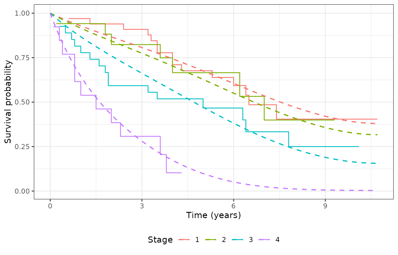
Kaplan-Meier by stage (steps) vs Bernstein PH at median age (smooth dashed).
Visual check — forest plot
td <- tidy(fit, conf.int = TRUE, exponentiate = TRUE)
td$term <- factor(td$term, levels = rev(td$term))
ggplot(td, aes(x = estimate, y = term, xmin = conf.low, xmax = conf.high)) +
  geom_vline(xintercept = 1, linetype = "dashed", color = "grey50") +
  geom_pointrange(linewidth = 0.4) +
  labs(x = "Hazard ratio", y = NULL) +
  theme_bw()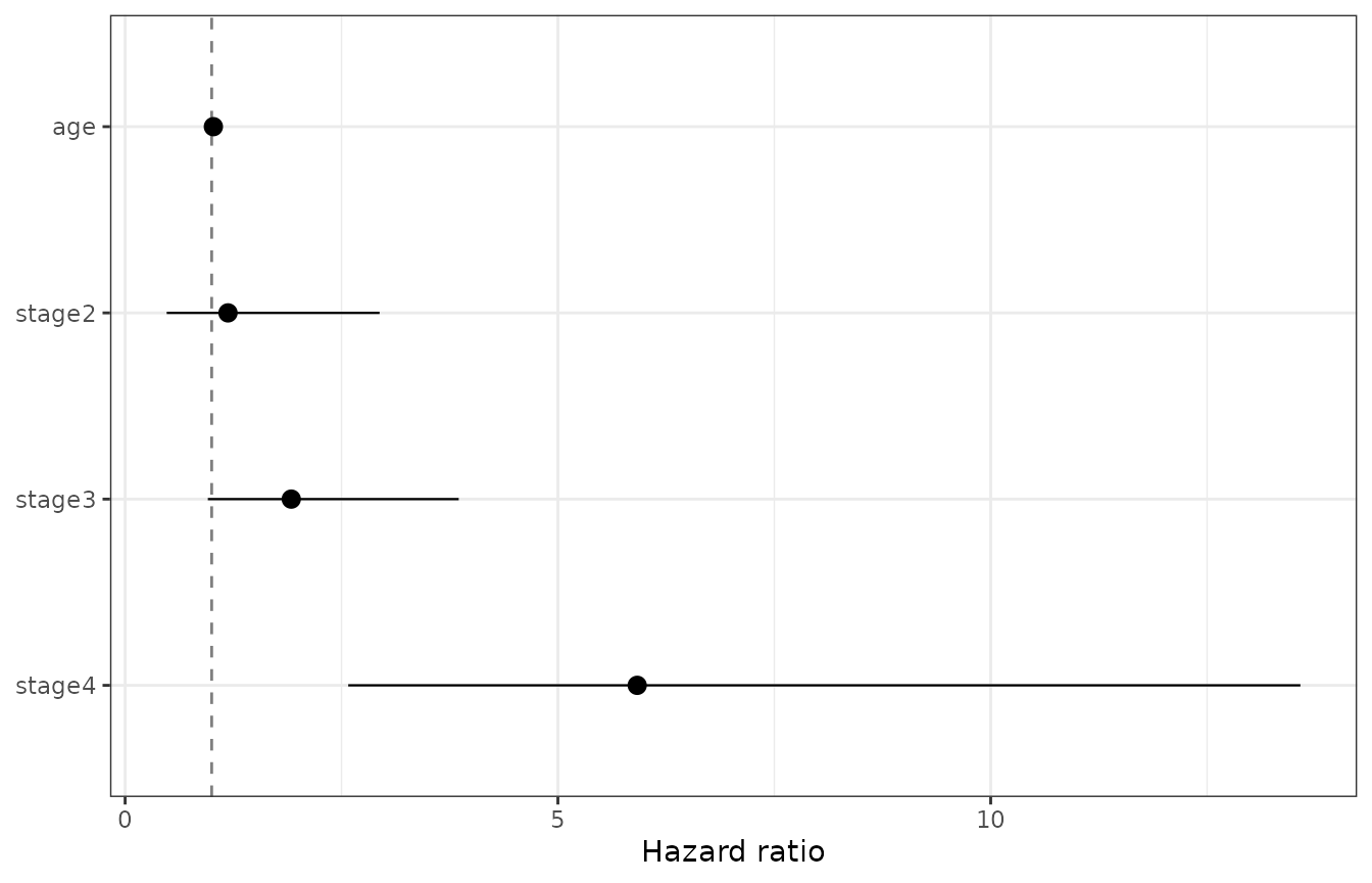
Exponentiated coefficients (hazard ratios) with 95% CIs.
Printing
print(fit, what = "summary")
#> Call:
#> bpph(formula = Surv(time, delta) ~ age + stage, degree = 5, data = larynx,
#>     approach = "mle", init = 0, model = "ph")
#>
#> Bernstein PH model:
#> Regression coefficients:
#>        Estimate    2.5%   97.5% Std. Error z value Pr(>|z|)
#> age      0.0197 -0.0084  0.0478     0.0143     1.4     0.17
#> stage2   0.1729 -0.7325  1.0783     0.4619     0.4     0.71
#> stage3   0.6521 -0.0450  1.3492     0.3557     1.8     0.07 .
#> stage4   1.7777  0.9469  2.6085     0.4239     4.2    3e-05 ***
#> ---
#> Signif. codes:  0 '***' 0.001 '**' 0.01 '*' 0.05 '.' 0.1 ' ' 1
#>
#> Exponentiated coefficients:
#>        Estimate 2.5% 97.5%
#> age        1.02 0.99   1.0
#> stage2     1.19 0.48   2.9
#> stage3     1.92 0.96   3.9
#> stage4     5.92 2.58  13.6
#>
#> ---
#> loglik = -141   AIC = 299