Inference and model comparison (MLE)

Maximum-likelihood fits support classical inference on the full Bernstein likelihood (not Cox partial likelihood).

Before you model

library(spsurv)
library(generics)
library(survival)
library(ggplot2)
data(veteran)

We compare a null model (intercept-only baseline) with a model including Karnofsky score — the same question as in the paper: is performance status worth including?

Fit and summarize

fit0 <- bpph(
  Surv(time, status) ~ 1,
  degree = 5,
  data = veteran,
  approach = "mle",
  init = 0
)
fit1 <- bpph(
  Surv(time, status) ~ karno,
  degree = 5,
  data = veteran,
  approach = "mle",
  init = 0
)
fit2 <- bpph(
  Surv(time, status) ~ karno + factor(celltype),
  degree = 5,
  data = veteran,
  approach = "mle",
  init = 0
)

td <- tidy(fit1, conf.int = TRUE, exponentiate = TRUE)
td
#>    term component  estimate   std.error statistic      p.value  conf.low
#> 1 karno      coef 0.9672297 0.005010139 -6.650367 2.923629e-11 0.9577783
#>   conf.high
#> 1 0.9767744

glance(fit1)
#>     n nevent    logLik approach model df statistic      p.value       rsq
#> 1 137    128 -724.8211      mle    ph  6  42.74605 6.232769e-11 0.2680294
#>     max.rsq      AIC      BIC
#> 1 0.9999814 1461.642 1479.162

Visual check — forest plot

td$term <- factor(td$term, levels = rev(td$term))
ggplot(td, aes(x = estimate, y = term, xmin = conf.low, xmax = conf.high)) +
  geom_vline(xintercept = 1, linetype = "dashed", color = "grey50") +
  geom_pointrange(linewidth = 0.4) +
  labs(x = "Hazard ratio", y = NULL) +
  theme_bw()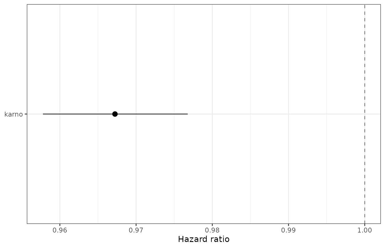

Karnofsky hazard ratio with 95% CI.

Visual check — model comparison

cmp <- data.frame(
  model = c("Null", "Karnofsky"),
  AIC = c(AIC(fit0), AIC(fit1)),
  logLik = c(as.numeric(logLik(fit0)), as.numeric(logLik(fit1))),
  df = c(attr(logLik(fit0), "df"), attr(logLik(fit1), "df"))
)
cmp
#>       model      AIC    logLik df
#> 1      Null 1502.388 -746.1941  5
#> 2 Karnofsky 1461.642 -724.8211  6

anova(fit0, fit1)
#> Analysis of Deviance Table
#> 
#> Bernstein PH model (MLE), n = 137, degree = 5
#>   Terms Resid. Df  -2*LL Test Df Deviance  Pr(>Chi)    
#> 1     1       132 1492.4    1                          
#> 2     2       131 1449.6    1  1   42.746 6.233e-11 ***
#> ---
#> Signif. codes:  0 '***' 0.001 '**' 0.01 '*' 0.05 '.' 0.1 ' ' 1
anova(fit1, fit2)
#> Analysis of Deviance Table
#> 
#> Bernstein PH model (MLE), n = 137, degree = 5
#>   Terms Resid. Df  -2*LL Test Df Deviance  Pr(>Chi)    
#> 1     1       131 1449.6    1                          
#> 2     2       128 1432.0    2  3   17.616 0.0005277 ***
#> ---
#> Signif. codes:  0 '***' 0.001 '**' 0.01 '*' 0.05 '.' 0.1 ' ' 1
anova(fit2)
#> Analysis of Deviance Table
#> 
#> Bernstein PH model (MLE), n = 137, degree = 5
#> 
#> Terms added sequentially (first to last)
#>                  Df Deviance Resid. Df  -2*LL  Pr(>Chi)    
#> NULL                               132 1492.4              
#> karno             1   42.746       131 1449.6 6.233e-11 ***
#> factor(celltype)  3   17.616       128 1432.0 0.0005277 ***
#> ---
#> Signif. codes:  0 '***' 0.001 '**' 0.01 '*' 0.05 '.' 0.1 ' ' 1

Pairwise comparisons report the likelihood-ratio statistic on the simpler model row. A single fitted model produces a sequential table (NULL, then each term in formula order), matching survival::survreg conventions.

Why this is insightful

Forest plots translate coefficients into decision-relevant effect sizes. The LR test and AIC answer whether Karnofsky improves fit enough to justify the extra regression parameter (Bernstein degree held constant).

What to decide

• HR CI excludes 1 and significant LR → include covariate.
• AIC favors complex model but effect negligible → balance parsimony vs fit.
• Compare models at the same Bernstein degree — df includes all gamma parameters.

Degrees of freedom (visual)

df_tbl <- data.frame(
  Quantity = c(
    "logLik() / AIC df",
    "summary() logtest df",
    "anova() nested df diff"
  ),
  fit0 = c(
    attr(logLik(fit0), "df"),
    "\u2014",
    "\u2014"
  ),
  fit1 = c(
    attr(logLik(fit1), "df"),
    summary(fit1)$logtest["df"],
    attr(logLik(fit1), "df") - attr(logLik(fit0), "df")
  ),
  Counts = c(
    "Regression + length(bp.param)",
    "Regression terms only",
    "Total parameter difference"
  )
)
df_tbl
#>                 Quantity fit0 fit1                        Counts
#> 1      logLik() / AIC df    5    6 Regression + length(bp.param)
#> 2   summary() logtest df    —    1         Regression terms only
#> 3 anova() nested df diff    —    1    Total parameter difference

Confidence intervals and variance

confint(fit1, level = 0.95)
#>              2.5%       97.5%
#> karno -0.04313896 -0.02349957

dim(vcov(fit1))
#> [1] 1 1
dim(vcov(fit1, bp.param = TRUE))
#> [1] 6 6

estimates(), se(), and extractAIC()

head(estimates(fit1))
#>         karno      gamma[1]      gamma[2]      gamma[3]      gamma[4] 
#> -0.0333192663 13.8798541589 11.4178267263 11.4086099336  0.0008454356 
#>      gamma[5] 
#> 17.0616750768
extractAIC(fit1)
#> [1]    6.000 1461.642

Null model

summary(fit0)
#> Call:
#> bpph(formula = Surv(time, status) ~ 1, degree = 5, data = veteran, 
#>     approach = "mle", init = 0, model = "ph")
#> 
#> 
#>          log(gamma)    gamma se(log(gamma))    z Pr(>z)    
#> gamma[1]    7.5e-01  2.1e+00        0.0e+00  Inf <2e-16 ***
#> gamma[2]   -1.2e+00  2.9e-01        3.9e+00  3.2  7e-04 ***
#> gamma[3]    5.2e-01  1.7e+00        8.8e-01 85.0 <2e-16 ***
#> gamma[4]   -1.2e+01  4.5e-06        5.2e+02  0.0    0.5    
#> gamma[5]    1.8e-01  1.2e+00        7.0e-01 74.4 <2e-16 ***
#> ---
#> Signif. codes:  0 '***' 0.001 '**' 0.01 '*' 0.05 '.' 0.1 ' ' 1
#> 
#> Loglik(model)=  -746   Loglik(baseline only)=  -746 
#> n=  137,  number of events=  128
logLik(fit0)
#> 'log Lik.' -746.1941 (df=5)