Survival prediction and ggplot workflows

Unlike stepwise Cox survfit curves, spsurv evaluates survival on a dense time grid using the fitted Bernstein baseline. This vignette connects observed Kaplan-Meier curves to model-based predictions.

Before you model

library(spsurv)
library(KMsurv)
library(survival)
library(ggplot2)
data(larynx)
larynx$stage <- factor(larynx$stage)

km_stage <- survfit(Surv(time, delta) ~ stage, data = larynx)
km_long <- data.frame(
  time = km_stage$time,
  surv = km_stage$surv,
  stage = rep(levels(larynx$stage), km_stage$strata)
)
ggplot(km_long, aes(x = time, y = surv, color = stage)) +
  geom_step(linewidth = 0.6) +
  geom_point(
    data = subset(larynx, delta == 0),
    aes(x = time, y = 0, color = stage),
    shape = 3,
    size = 1.5,
    alpha = 0.5,
    inherit.aes = FALSE
  ) +
  labs(x = "Time (years)", y = "Survival probability", color = "Stage") +
  theme_bw() +
  theme(legend.position = "bottom")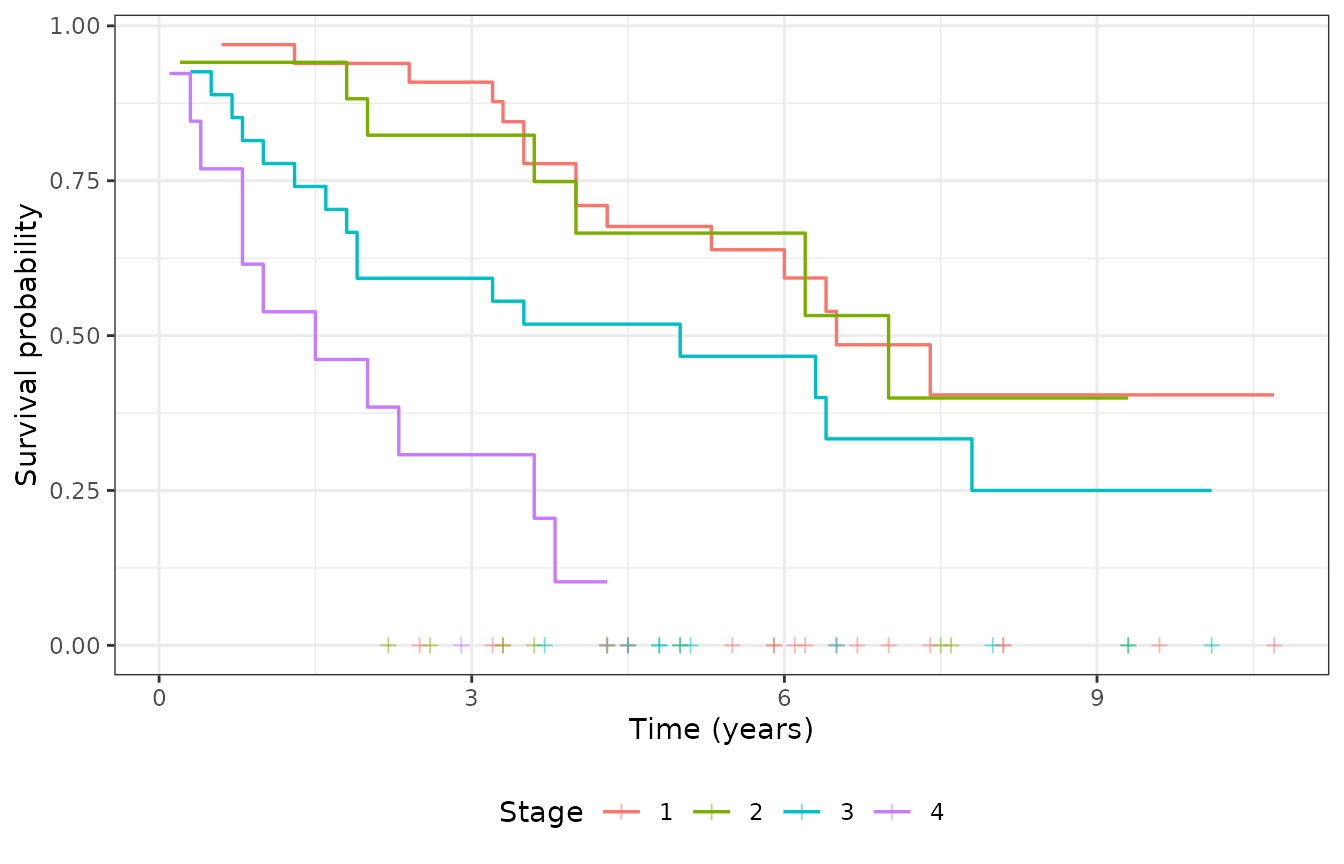

Kaplan-Meier by stage with censoring marks (+).

We compare predictions at age = 70 across all stages — a clinically interpretable profile that holds age fixed while varying disease stage.

Why this is insightful

KM curves show unadjusted stage separation. Censoring marks (+) remind you that late follow-up estimates rest on fewer subjects.

What to decide

Clear stage ordering in KM → including stage in the model is justified.
Crossing KM curves → proportional hazards may be questionable; see the Choosing PH, PO, and AFT models vignette.

Fit and summarize

fit <- bpph(
  Surv(time, delta) ~ age + stage,
  degree = 5,
  data = larynx,
  approach = "mle",
  init = 0
)
summary(fit)
#> Call:
#> bpph(formula = Surv(time, delta) ~ age + stage, degree = 5, data = larynx, 
#>     approach = "mle", init = 0, model = "ph")
#> 
#> Bernstein PH model: 
#> Regression coefficients:
#>        Estimate    2.5%   97.5% Std. Error z value Pr(>|z|)    
#> age      0.0197 -0.0084  0.0478     0.0143     1.4     0.17    
#> stage2   0.1729 -0.7325  1.0783     0.4619     0.4     0.71    
#> stage3   0.6521 -0.0450  1.3492     0.3557     1.8     0.07 .  
#> stage4   1.7777  0.9469  2.6085     0.4239     4.2    3e-05 ***
#> ---
#> Signif. codes:  0 '***' 0.001 '**' 0.01 '*' 0.05 '.' 0.1 ' ' 1
#> 
#> Exponentiated coefficients:
#>        Estimate 2.5% 97.5%
#> age        1.02 0.99   1.0
#> stage2     1.19 0.48   2.9
#> stage3     1.92 0.96   3.9
#> stage4     5.92 2.58  13.6
#> 
#> --- 
#> loglik = -141   AIC = 299

Prediction grid

plot_times <- seq(0, max(larynx$time), length.out = 121)
newdata <- data.frame(age = 70, stage = levels(larynx$stage))
newdata
#>   age stage
#> 1  70     1
#> 2  70     2
#> 3  70     3
#> 4  70     4

`predict()` — tidy data frame

pr <- predict(fit, newdata = newdata, times = plot_times)
head(pr)
#>     age stage id       time      surv     lower upper      cumhaz    std.err
#> 1    70     1  1 0.00000000 1.0000000 1.0000000     1 0.000000000 0.00000000
#> 1.1  70     1  1 0.08916667 0.9922916 0.9665815     1 0.007738282 0.01339380
#> 1.2  70     1  1 0.17833333 0.9847495 0.9390069     1 0.015367968 0.02426802
#> 1.3  70     1  1 0.26750000 0.9773649 0.9160475     1 0.022895223 0.03305766
#> 1.4  70     1  1 0.35666667 0.9701290 0.8965413     1 0.030326268 0.04024799
#> 1.5  70     1  1 0.44583333 0.9630332 0.8793507     1 0.037667370 0.04638049

Visual check — KM vs model overlay

Panel A: observed KM (step) vs model prediction (dashed) per stage.

curve_labs <- paste("Stage", newdata$stage)
pr$series <- curve_labs[match(as.character(pr$id), as.character(seq_len(nrow(newdata))))]

ggplot() +
  geom_step(
    data = km_long,
    aes(x = time, y = surv, color = stage),
    linewidth = 0.5,
    alpha = 0.8
  ) +
  geom_line(
    data = pr,
    aes(x = time, y = surv, color = series),
    linetype = "dashed",
    linewidth = 0.6
  ) +
  labs(x = "Time (years)", y = "Survival probability", color = NULL) +
  theme_bw() +
  theme(legend.position = "bottom")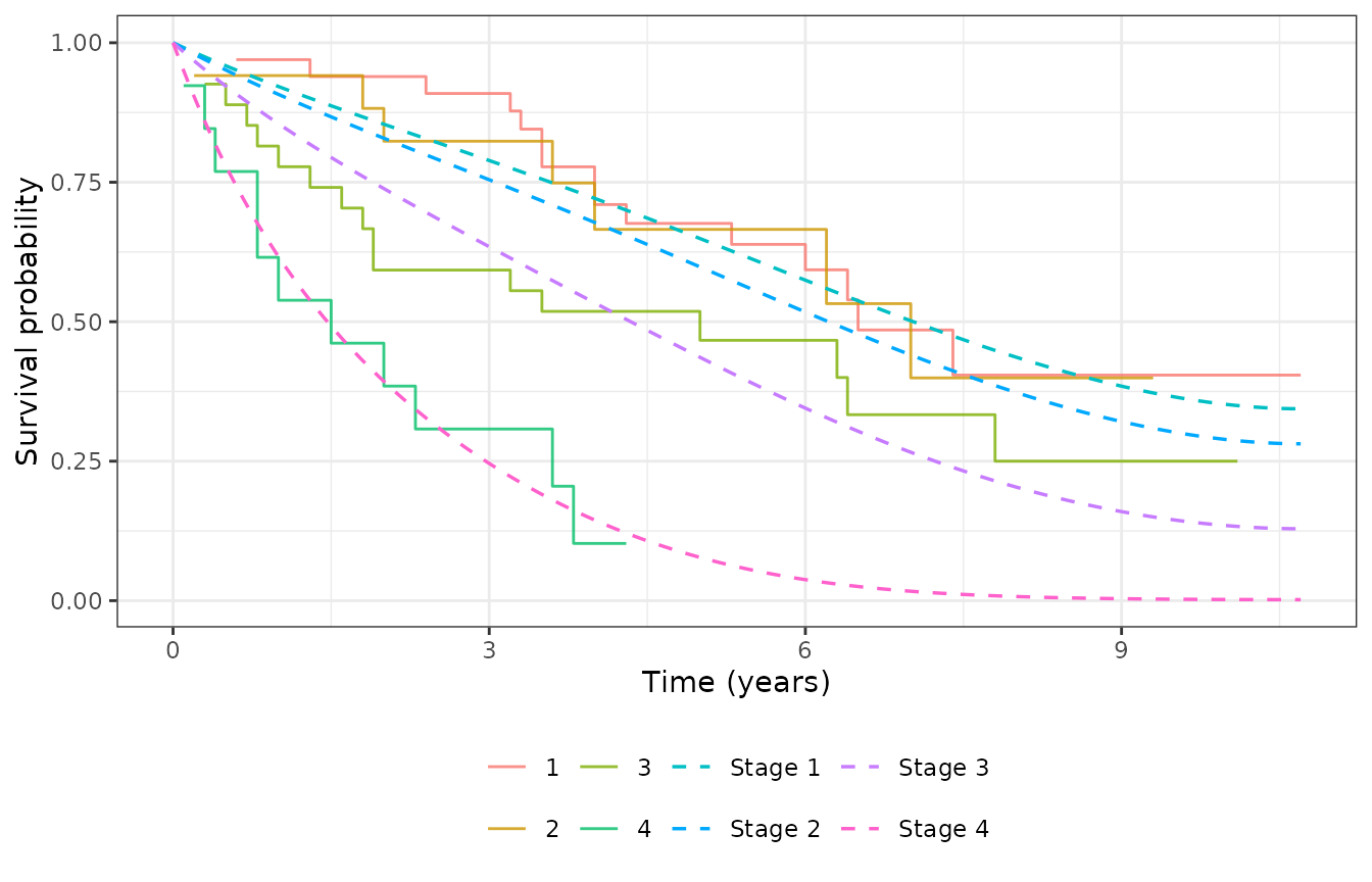

Observed KM (solid) vs model prediction at age 70 (dashed).

Panel B: model-based ribbons (adjusted prediction with uncertainty).

ggplot(pr, aes(x = time, y = surv, color = series, fill = series)) +
  geom_ribbon(aes(ymin = lower, ymax = upper), alpha = 0.2, colour = NA) +
  geom_line(linewidth = 0.5) +
  labs(x = "Time (years)", y = "Survival probability", color = NULL, fill = NULL) +
  theme_bw() +
  theme(legend.position = "bottom")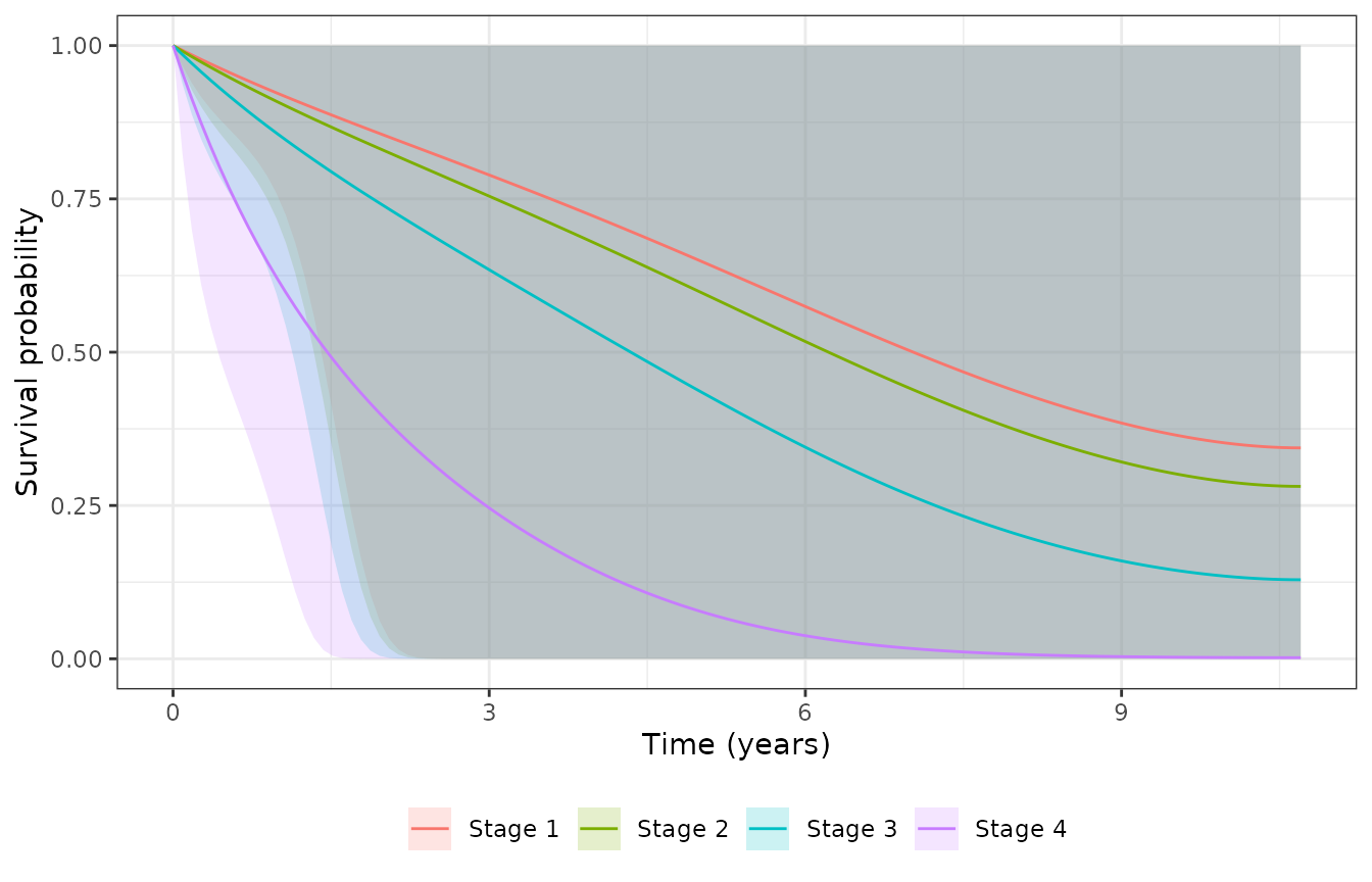

Stage-specific survival curves with 95% intervals.

Why this is insightful

Panel A connects the smooth BP fit to observed risk sets. Panel B shows covariate-adjusted uncertainty — ribbons often widen late in follow-up when data are sparse.

What to decide

Model curves systematically below KM → check covariate adjustment or misspecification.
Wide bands late in follow-up → avoid over-interpreting tail survival.
For publication → export predict() output directly to your ggplot pipeline.

`survfit()` with `tidy = TRUE`

sf <- survfit(fit, newdata = newdata, times = plot_times, tidy = TRUE)
head(sf)
#>     age stage id       time      surv     lower upper      cumhaz    std.err
#> 1    70     1  1 0.00000000 1.0000000 1.0000000     1 0.000000000 0.00000000
#> 1.1  70     1  1 0.08916667 0.9922916 0.9665815     1 0.007738282 0.01339380
#> 1.2  70     1  1 0.17833333 0.9847495 0.9390069     1 0.015367968 0.02426802
#> 1.3  70     1  1 0.26750000 0.9773649 0.9160475     1 0.022895223 0.03305766
#> 1.4  70     1  1 0.35666667 0.9701290 0.8965413     1 0.030326268 0.04024799
#> 1.5  70     1  1 0.44583333 0.9630332 0.8793507     1 0.037667370 0.04638049

Bayesian fits

For approach = "bayes", credible bands use posterior draws with interval.type = "hpd" and monotone = TRUE (default for Bayes).

fit_bayes <- bpph(
  Surv(time, delta) ~ age + stage,
  degree = 5,
  data = larynx,
  approach = "bayes",
  iter = 400,
  chains = 1,
  cores = 1
)
predict(fit_bayes, newdata = newdata, times = plot_times, interval.type = "hpd")

Interval types (MLE)

Log–log intervals are undefined at S = 1 (time = 0), so we evaluate at time > 0 only:

loglog_times <- plot_times[plot_times > 0]
head(predict(fit, newdata = newdata, times = loglog_times, type = "log-log"))
#>     age stage id       time      surv     lower     upper      cumhaz
#> 1    70     1  1 0.08916667 0.9922916 0.7944418 0.9997398 0.007738282
#> 1.1  70     1  1 0.17833333 0.9847495 0.7121628 0.9993045 0.015367968
#> 1.2  70     1  1 0.26750000 0.9773649 0.6784516 0.9986497 0.022895223
#> 1.3  70     1  1 0.35666667 0.9701290 0.6644510 0.9977528 0.030326268
#> 1.4  70     1  1 0.44583333 0.9630332 0.6565284 0.9966338 0.037667370
#> 1.5  70     1  1 0.53500000 0.9560693 0.6470954 0.9953739 0.044924834
#>        std.err
#> 1   0.01339380
#> 1.1 0.02426802
#> 1.2 0.03305766
#> 1.3 0.04024799
#> 1.4 0.04638049
#> 1.5 0.05205317

Before you model

Why this is insightful

What to decide

Fit and summarize

Prediction grid

predict() — tidy data frame

Visual check — KM vs model overlay

Why this is insightful

What to decide

survfit() with tidy = TRUE

Bayesian fits

Interval types (MLE)

`predict()` — tidy data frame

`survfit()` with `tidy = TRUE`