Compute survival curves for a fitted spbp model.
Usage
# S3 method for class 'spbp'
survfit(
  formula,
  newdata = NULL,
  times = NULL,
  se.fit = TRUE,
  interval = 0.95,
  type = c("log", "log-log", "plain"),
  interval.type = c("hpd", "quantile"),
  monotone = NULL,
  tidy = FALSE,
  baseline = FALSE,
  ...
)

# S3 method for class 'survfitbp'
as.data.frame(x, row.names = NULL, optional = FALSE, ...)

# S3 method for class 'survfitbp'
plot(
  x,
  conf.int,
  col = 1,
  lty = 1,
  lwd = 1.5,
  xlab = "Time",
  ylab = "Survival probability",
  ylim = c(0, 1),
  mark.time = FALSE,
  ...
)
Arguments
- formula
An object of class
"spbp"returned byspbp.- newdata
Optional data frame used to obtain survival curves for specific covariate values.
- times
Optional evaluation times: a
Survobject (legacy), or a non-negative numeric vector (unique values are used; suitable for smoothggplot2::geom_lineplots viapredict.spbporas.data.frame.survfitbp).- se.fit
Logical; if
TRUE, compute standard errors.- interval
Confidence level for intervals (e.g.
0.95).- type
Character; confidence interval transformation. One of
"log","log-log", or"plain".- interval.type
For Bayesian fits only:
"hpd"(default) or"quantile"(equal-tailed).- monotone
Logical; for Bayesian fits, enforce non-increasing credible-band limits over time so ribbons plot smoothly with
ggplot2::geom_line. Defaults toTRUEwhenapproach = "bayes".- tidy
Logical; if
TRUE, return adata.framefor ggplot2. instead of a"survfit"object.- baseline
Logical; if
TRUE, return the baseline survival curve \(S_0(t)\) at observed event times (ortimes) with no covariate effect. Whentidy = TRUE, returns a simpledata.framewith columnstimeandsurv.- ...
Further arguments passed to
survfit.coxphfor the reference Cox object (e.g.conf.typeis ignored; usetypeinstead).- x
Object from
survfit.spbp.- row.names, optional
Unused; included for S3 consistency.
- conf.int
Logical; draw pointwise interval limits. Defaults to
TRUEfor a single curve when limits are present.- col, lty, lwd, xlab, ylab, ylim
Graphical parameters.
- mark.time
Ignored (Bernstein curves are continuous).
Value
An object of class "survfit" (with classes survfitbp, survfitcox, survfit).
A data.frame with columns id (curve index), time, surv,
lower, upper, cumhaz, std.err.
Functions
as.data.frame(survfitbp): Tidy survival curves forggplot2::geom_line/geom_ribbon.plot(survfitbp): Plot Bernstein-polynomial survival as a smooth line (type = "l"), never a Kaplan–Meier step function. Passconf.int = TRUEfor pointwise bands (also drawn with lines).
See also
spbp, survfit,
predict.spbp, survfit.spbp (as.data.frame method).
Examples
library(spsurv)
data(veteran, package = "survival")
#> Warning: data set ‘veteran’ not found
fit <- bpph(Surv(time, status) ~ karno + factor(celltype), data = veteran)
survfit(fit)
#> Call: survfit.spbp(formula = fit)
#>
#> n events median 0.95LCL 0.95UCL
#> [1,] 137 128 77.5 43.1 NA
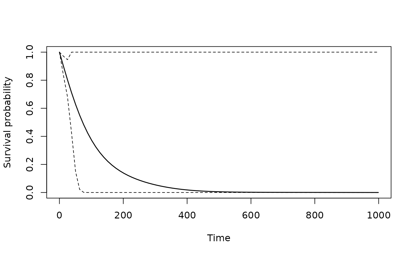
plot(survfit(fit, times = seq(0, max(veteran$time), length.out = 80)))
 data(veteran, package = "survival")
#> Warning: data set ‘veteran’ not found
fit <- bpph(Surv(time, status) ~ karno, data = veteran, approach = "mle", init = 0)
sf <- survfit(fit, times = seq(0, max(veteran$time), length.out = 80))
#> Warning: Bernstein-polynomial (gamma) information matrix is ill-conditioned (kappa = 1.04e+12, degree = 12); delta-method survival standard errors and confidence bands may be unreliable. Try refitting with a lower Bernstein degree (argument `degree` to bpph(), bppo(), bpaft(), or spbp()).
head(as.data.frame(sf))
#> id time surv lower upper cumhaz std.err
#> 1 1 0.00000 1.0000000 1.0000000000 1 0.0000000 0.00000000
#> 2 1 12.64557 0.8947161 0.7998515928 1 0.1112489 0.05718484
#> 3 1 25.29114 0.7912094 0.4045850767 1 0.2341926 0.34220047
#> 4 1 37.93671 0.6947400 0.0887711859 1 0.3642176 1.04975170
#> 5 1 50.58228 0.6079767 0.0068732687 1 0.4976187 2.28703019
#> 6 1 63.22785 0.5317991 0.0001672713 1 0.6314896 4.11456738
data(veteran, package = "survival")
#> Warning: data set ‘veteran’ not found
fit <- bpph(Surv(time, status) ~ karno, data = veteran, approach = "mle", init = 0)
sf <- survfit(fit, times = seq(0, max(veteran$time), length.out = 80))
#> Warning: Bernstein-polynomial (gamma) information matrix is ill-conditioned (kappa = 1.04e+12, degree = 12); delta-method survival standard errors and confidence bands may be unreliable. Try refitting with a lower Bernstein degree (argument `degree` to bpph(), bppo(), bpaft(), or spbp()).
head(as.data.frame(sf))
#> id time surv lower upper cumhaz std.err
#> 1 1 0.00000 1.0000000 1.0000000000 1 0.0000000 0.00000000
#> 2 1 12.64557 0.8947161 0.7998515928 1 0.1112489 0.05718484
#> 3 1 25.29114 0.7912094 0.4045850767 1 0.2341926 0.34220047
#> 4 1 37.93671 0.6947400 0.0887711859 1 0.3642176 1.04975170
#> 5 1 50.58228 0.6079767 0.0068732687 1 0.4976187 2.28703019
#> 6 1 63.22785 0.5317991 0.0001672713 1 0.6314896 4.11456738