This vignette shows how to export structured results
from interactmeta for quality control,
reporting, or downstream tables. The idea matches “calculate
once, use many times”: fit the model, then take all display
numbers from tidy() (and comparison
helpers), not from re-typing forest-plot labels.
Getting started with cams(): vignette("cams").
Setup and fits
We use the steroids IV/NIV example
(same data path as vignette("cams")).
CAMS uses method = "REML"
here; sensitivity analyses add DA, AD,
and SWADA.
library(interactmeta)
library(dplyr)
#>
#> Attaching package: 'dplyr'
#> The following objects are masked from 'package:stats':
#>
#>     filter, lag
#> The following objects are masked from 'package:base':
#>
#>     intersect, setdiff, setequal, union

steroids_obs <- steroids |> filter(n > 0)
steroids_es <- escalc(
  measure = "OR",
  ai = treat.events,
  bi = treat.total - treat.events,
  ci = cont.events,
  di = cont.total - cont.events,
  data = steroids_obs
)
des <- ifrac(steroids_es, reference = "NIV")

fit_cam <- cams(des, reference = "NIV", method = "REML")
fit_da <- da(des, reference = "NIV", method = "REML")
fit_ad <- ad(des, reference = "NIV", method = "REML")
fit_sw <- swada(des, reference = "NIV", method = "REML")
Canonical export: tidy(fit)
tidy(fit) binds interaction, modifier,
combined, and (optionally) heterogeneity rows in one tibble. You can
still call tidy(interactions(...)) when
you need a single estimand. Typical columns:
| Column | Meaning |
|---|---|
estimate,
std.error,
conf.low,
conf.high
|
Point and interval on the requested scale |
type |
e.g. Overall,
Prediction
|
subgroup /
level
|
Modifier label ( modifiers() ) |
interaction |
Contrast label ( interactions() ) |
parameter,
label
|
Heterogeneity summaries (
heterogeneity() ) |
results <- tidy(
  fit_cam,
  estimands = c("interaction", "modifiers", "combined", "heterogeneity"),
  type = "Overall",
  exponentiate = TRUE
)
knitr::kable(
  results |>
    filter(estimand != "heterogeneity", type == "Overall") |>
    select(estimand, level, interaction, type, estimate, conf.low, conf.high),
  digits = 2
)| estimand | level | interaction | type | estimate | conf.low | conf.high |
|---|---|---|---|---|---|---|
| interaction | IV-NIV | IV-NIV | Overall | 1.35 | 0.32 | 2.38 |
| modifier | IV | NA | Overall | 1.47 | 0.78 | 2.77 |
| modifier | NIV | NA | Overall | 0.38 | 0.18 | 0.82 |
| combined | NA | NA | Overall | -0.16 | -1.72 | 1.39 |
Add run metadata once (reference, inference, reporting IF) for audit trails:
meta <- tibble::tibble(
  package = "interactmeta",
  method = "CAMS",
  inference = "REML",
  reference = "NIV",
  scale = "OR",
  reporting_if = as.numeric(ifrac(fit_cam, ifrac = "interaction"))
)
knitr::kable(meta, digits = 3)| package | method | inference | reference | scale | reporting_if |
|---|---|---|---|---|---|
| interactmeta | CAMS | REML | NIV | OR | 0.593 |
Pre-specified sensitivity analyses
sensitivity() fits DA,
AD, SWADA, and CAMS
on the same data; compare() aligns them on
one table—useful as sensitivity rows in a report (not
as a single “consensus” estimate).
sens <- sensitivity(des, reference = "NIV", method = "REML", silent = 2)
cmp_ix <- compare(
  sens,
  estimand = "interaction",
  exponentiate = TRUE,
  type = "Overall"
)
knitr::kable(cmp_ix, digits = 2, caption = "Interaction OR: construction sensitivity")| approach | contrast | estimate | se | ci.lb | ci.ub |
|---|---|---|---|---|---|
| DA | IV - NIV (DA) | 1.96 | 0.86 | 0.83 | 4.62 |
| AD | IV - NIV | 3.86 | 2.02 | 1.38 | 10.78 |
| SWADA | IV - NIV | 3.86 | 2.02 | 1.38 | 10.78 |
| CAMS | IV - NIV | 1.35 | 0.52 | 0.32 | 2.38 |
cmp_sg <- compare(
  sens,
  estimand = "modifiers",
  exponentiate = TRUE,
  type = "Overall"
)
knitr::kable(cmp_sg, digits = 2, caption = "Modifier ORs: DA vs SWADA vs CAMS")| approach | subgroup | estimate | se | ci.lb | ci.ub |
|---|---|---|---|---|---|
| DA | NIV | 0.41 | 0.16 | 0.19 | 0.88 |
| SWADA | NIV | 0.38 | 0.15 | 0.17 | 0.84 |
| CAMS | NIV | 0.38 | 0.15 | 0.18 | 0.82 |
| DA | IV | 0.79 | 0.15 | 0.55 | 1.15 |
| SWADA | IV | 1.47 | 0.49 | 0.76 | 2.83 |
| CAMS | IV | 1.47 | 0.47 | 0.78 | 2.77 |
Note. Under default weights, SWADA matches AD for the interaction; both appear in the interaction sensitivity table because they answer different construction definitions.
QC: one row lookup vs the printed summary
QC should recover the same Overall interaction as
print() /
interactions():
Handoff to layout tools
interactmeta does not render regulatory
TLGs. After tidy(), use your table package
of choice (gt,
gtsummary,
flextable, …) on the tibble. Keep
computation (this export) separate from
layout, in line with CDISC Analysis Results
Data thinking: structured statistics first, formatted output
second.
Minimal gt example (skip if
gt is not installed):
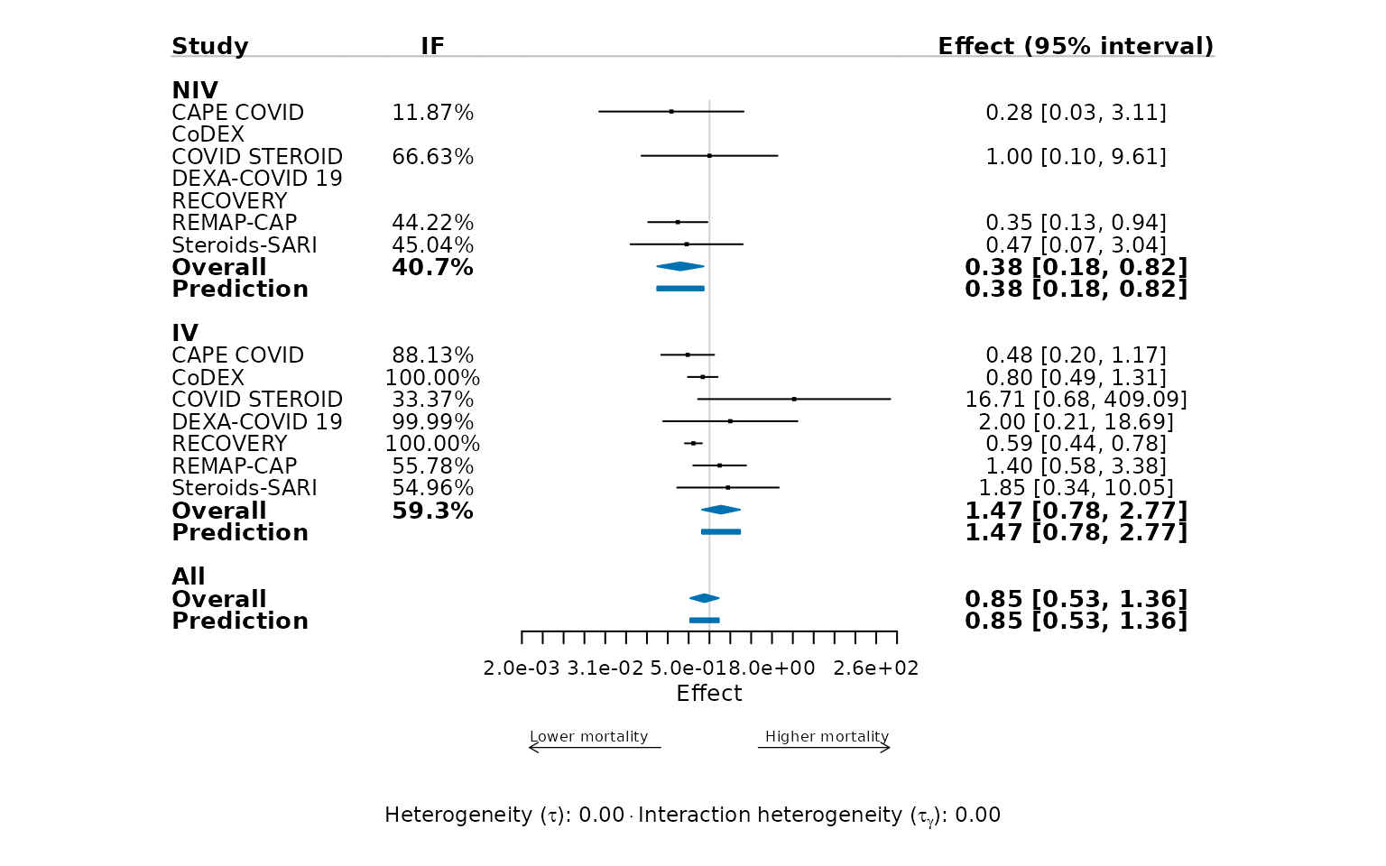
Forest plots and exported numbers
Pooled Overall diamonds on
forestplot(fit_cam) match
modifiers() /
combined() at the reporting IF shown under
the axis. When QC fails, check
exponentiate,
type, and
reference match between the plot and
tidy() calls.
forestplot(
  fit_cam,
  exponentiate = TRUE,
  favours = c("Lower mortality", "Higher mortality")
)
Related reading
-
vignette("cams")— estimands, assumptions, Bayesian vs REML. -
vignette("worked-examples")—age,edss, and other shipped tables.